The 3D model you built is a physical model with actual member size rendered visually. The analysis converts the physical model into the analytical model (as shown below).
The analytical model is essentially a centre-line wireframe model. For members to be connected properly, the analytical wire frame must meet a common joint. Joints are insertion points created at intersection of axes.
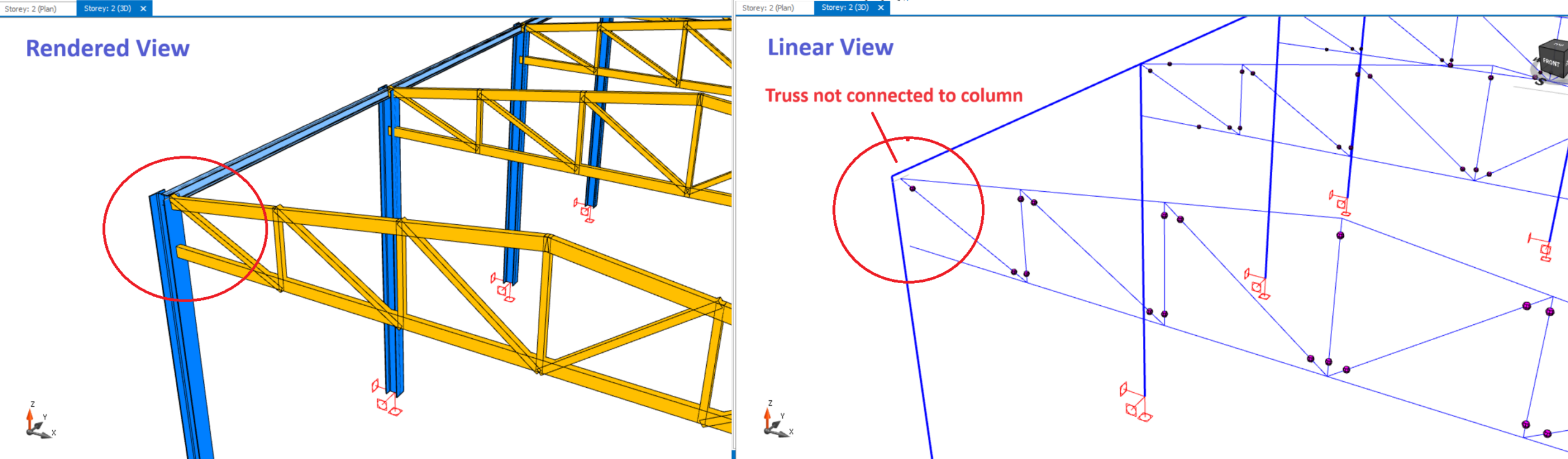
Hence, when modelling, you need to ensure that members are using common axes or intersection of axes for members to be connected. Merely checking the 3D rendered view does not confirm whether members are connected analytically.
Preview of Analytical Model using Linear view
For reasons stated above, it is important to check member connectivity before the analysis, otherwise analysis may fail or yield many warning message of instability.
To display and verify the analytical model before the analysis :
1. Create a 3D view > By default a "Solid" or "Rendered" model is shown
2. Press "CTRL + D" consecutively > this will cycle to various Display Style (Rendered, Flat, Hidden Line, Linear)
3. Ensure "Linear" is active > This shows the 3D analytical wireframe model
Alternatively, in 3D view, click on "Linear" icon just above the Structure tree (as below)
4. Verify the members are connected properly by zooming in common joints of interest.
Below is an example where members are not connected analytical but appears to be connected in solid rendered view.
–> Click to enlarge picture
For steel structure, we highly recommend you model all steel members in Linear view. This will ensure all members are connected properly, as modelling in physical view will likely result in non-connectivity of steel members.
You can also select a group of members and display the linear view of those selected members only :
1. Select the members you want to view in wireframe mode
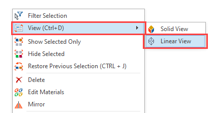
2. Choose the "View > Linear View" command fromthe right-click menu.
3. The selected elements will begin to be displayed in wireframe mode.
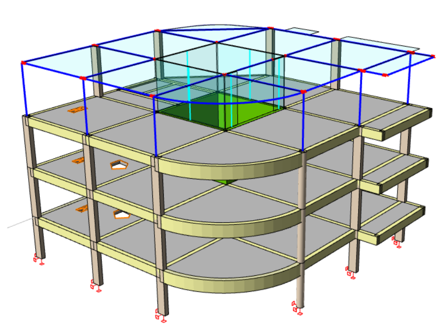
This way, you will obtain a hybrid view showing how the elements are connected to each other, example as below.
Once you have verified the connectivity of members, you can proceed to run Building Analysis with confidence.
Display Analytical Model
The Building Analysisprocedure creates a 3D analytical model of the building, apply the loads and evaluates the member forces.
Go to the Analysis top ribbon, click on Analytical Model icon. If you have performed Finite Element Floor and Foundation analysis as well, then clicking “Analytical Model” button will prompt you with two options:
In Building Analysis Model, you can review the analysis results such as displacements, axial forces, shears, bending moments, torsions, and finite element contours.
Building Analysis Analytical Model
Once Building Analysis is completed successfully, you can access the detail Analytical Model, where you can check :
Whether the actual analytical model is prepared correctly
Display details such as frame and nodal loading, system connectivity information, rigid end zones, end releases etc.
Display deflections of members and shells
Display member forces, e.g axial load, shear & moments
The example below shows the Analytical Model of a 5 storey reinforced concrete building where the floor slabs are exclude included and not meshed.
The example below shows the Analytical Model of the same 5 storey reinforced concrete building where the floor slabs are included and meshed using finite element shells.
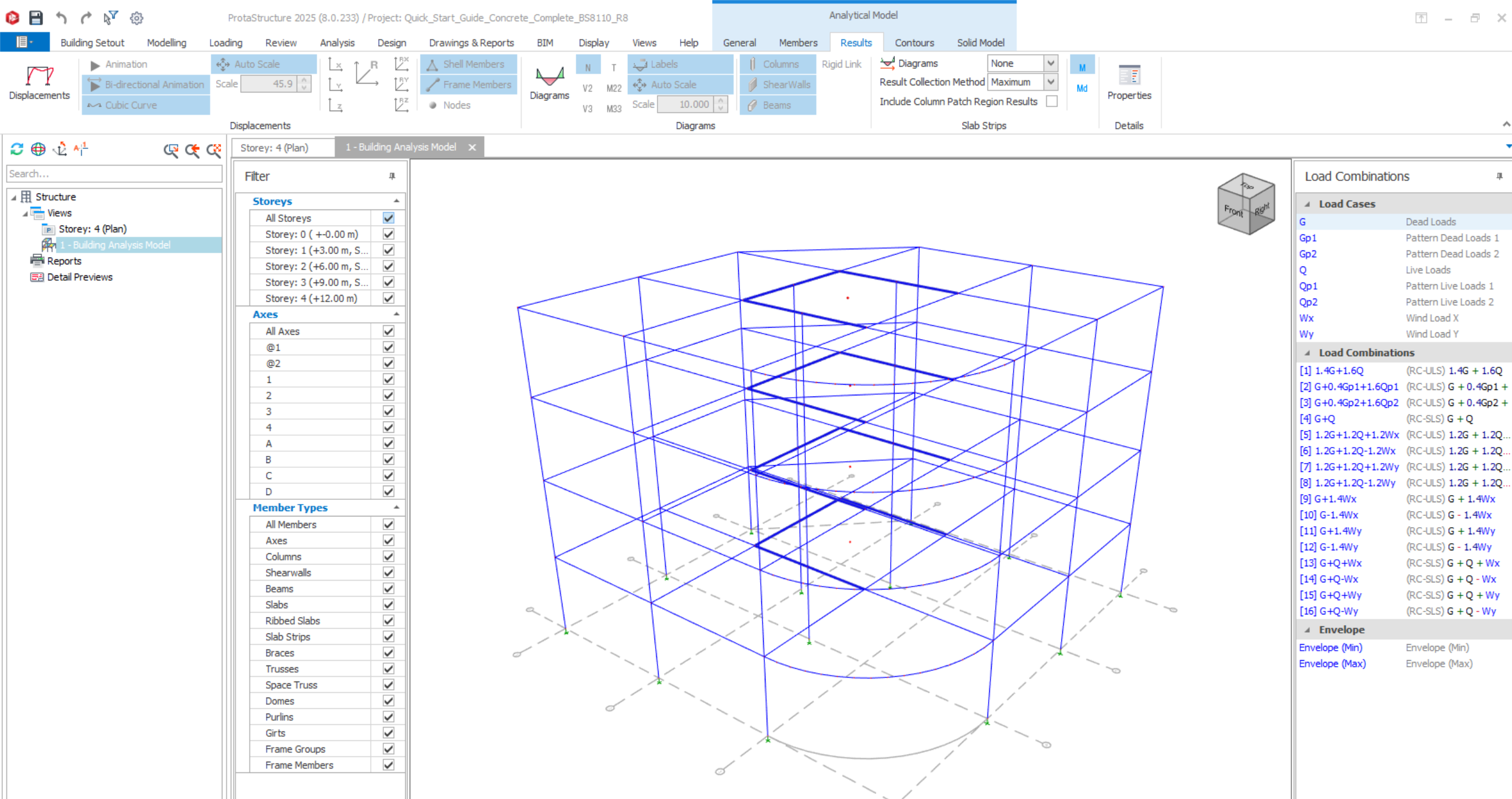
Filter Panel – Users can filter storeys, axes and member types to be shown in the analytical model.
Effects Panel – This panel would be available when users enable "Contours" after performing Building Analysis with Floor Meshed.
Load Combinations Panel – All load cases and load combinations will be shown here. Effects or forces diagram shown in analytical model will be based on selected load cases or load combinations here.
General Tab
The most commonly used view settings can be selected directly from the drop down menus, however other settings such as node display type, text properties and size, local axis colours etc. can be adjusted by displaying the “General” tab.
Settings
This button will display the "Analytical Model Settings" where you can adjust settings such as background color & settings related to node, frame, shell, diagram, displacement.
Plan
Set and lock viewing to plan view only.
View
Show the 3D viewing cube where you can click on face or corner of cube to set viewing direction.
Zoom in & Out
Self explanatory. Use mouse wheel can also zoom in & out
Orthogonal
Toggle between Orthogonal or Perspective 3D view.
Perspective requires more computing resources and may impact performance
Orthogonal requires less memory resources and can improve performance.
Increase / Decrease Font Size
Click to increase or decrease font size of text shown
Save / Copy Picture
Save picture as png file or copy it into memory, to be pasted elsewhere.
Find Node/Frame/Shell
This button can be used to locate an individual node, frame element or shell element within the 3-D analytical model.
This function is helpful in ascertain unstable members or joints in analytical model.
"Frame Loads" displays Point loads, distributed loads and user-defined loads acting on beam can be displayed on analytical model.
Frame Loads Labels
Shows values of frame loads.
Shell Elements
When Shell button is depressed the additional options will become active :
" Labels” to view the shell numbers.
"Shrink” to isolate shell elements from neighboring members and easily distinguish the connectivity information.
"Surface" to color / shade shells
"Thickness" to show shell thickness
"Pressure" to show decomposed pressure loads on shell
"Local Axis" to show 3 direction local axes of shell
"Solid Model" to render actual physical element with exact thickness.
Focus on Selected Members Only
Enables you to view frame elements results (displacement or forces diagrams) for selected frame only (while results of other elements will be hidden)
Applies only to frame elements (beam, column, mid-pier wall) and not shell elements, by these steps :
1. Activate this button
2. In Results tab, activate "Displacement" and / or force "Diagram" (N, V, T, M).
3. Select one or multiple frame member, i.e. beam, column or shell wall.
Step 2 & 3 can be reversed.
Show Member Tooltips
When the mouse is hover over a shell member, tooltip windows with connectivity information and analysis result for the selected shell member will appear.
Results Tab
Displacements, Frame Element Results and Contours are displayed for the load case selected in the “Loading”list.
If an eigenvalue analysis has been performed, mode shapes of the building will have been calculated and the modes can be selected from the “Loading” list in order to see the mode shape.
Displacements
Translation and rotation values at the node points can be displayed either as a resultant or in each of the global directions. For angled systems, if non-orthogonal displacements are to be investigated, then the “Resultant”option can be used. To animate the displacement display, select “Animation”.
The decimal precision of the displacement values can be adjusted from “Unit and Format” in the “Settings Center” .
Displacement is set to "Auto Scale" by default. To adjust the scale of displacement, uncheck the “Auto Scale”box and enter a value manually into the “Scale” field.
The “Cubic Curve”option draws the displacements of frame and shell members by making use of the loading on the elements, otherwise displacements are drawn just at the node points if this option is removed.
Animation
Click to animate the displaced shape for better visualization. This is particular useful to confirm whether members are connected properly. If they are not, it will be obvious they will displaced as separate entities.
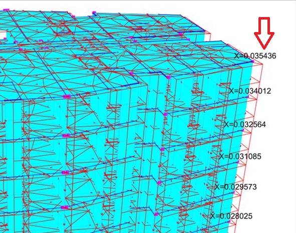
Displacement Values
Click to show actual displacement values. The legend is as follows :
X = Global horizontal plan displacement.
Y = Global vertical plan displacement.
Z = Global displacement along the storey height.
R = Resultant value in 3D space
Rx, Ry, & Rz are rotation, of joints in radians.
Diagrams
There are 6 force and moment components related to a frame element each of which can be displayed from the drop down menu:
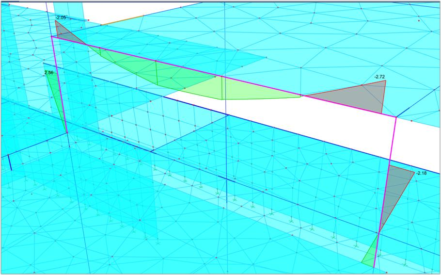
N : Axial Load. Negative value = Compression. Positive value = Tension.
T :Torsional Moment
V2 : Shear force along element local axis 2 (Major shear of beam and wall; shear of column in dir 2)
V3 : Shear forces along element local axis 3 (Minor shear of beam and wall; shear of column in dir 3)
M22 : Bending moments about element local axis 2 (Minor moment of beam and wall; moment of column about dir 2)
M33 :Bending moments about element local axis 3 (Major moment of beam and walls; moment of column about dir 3) Select the “Labels”option to see the diagram values on the display.
Moment or force diagrams are also drawn for the rigid members if you check the “Rigid Members” in the Diagrams section of the “View Settings” menu.
Diagrams are assigned an automatic scale when first loaded. Uncheck “Auto Scale”box in the “View Settings” menu and enter a value manually into the “Scale” field to use a different scale.
Rigid Link
To view the bending moment and forces in the rigid link, user need to click on Diagrams and click on Rigid Link tab.
Show Magnified Seismic Design Results
Magnified seismic design forces refer to the increased earthquake forces experienced by a structure during an earthquake, beyond what’s calculated from a linear elastic analysis.
Show Live Load Reduced Combination Results
Show combination forces with live load reduction applied
Slab Strips
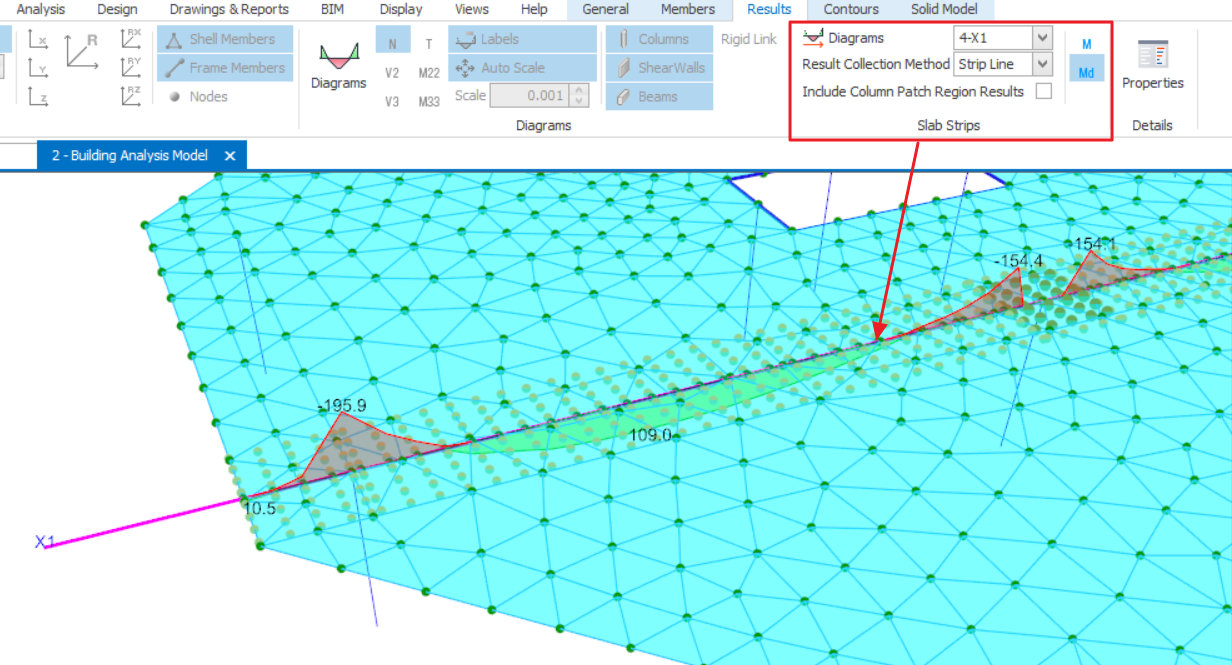
By default, “Diagrams” pull down menu in the “Slab Strips” ribbon group is disabled.
This button is only available when FE Slab Strip is modelled.
Users can choose to display moment diagram for one slab strip only or all slab strips in X or Y direction.
Md = Wood-Armer Effects is turned on
M = Wood-Armer Effects is Ignored
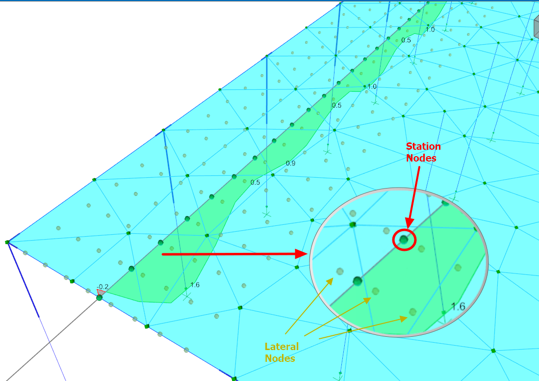
Result Collection Method for slab strips :
Maximum – The maximum of the lateral nodes at each station.
Integral – Integral is calculated from the integral of those nodes.
Strip Line – Only displays the values at the station nodes and lateral nodes are not considered.
Include Column Patch Region Results :
When this option is checked the results inside the patch panels will be included in the FE Fixed Band Strip diagram. You can notice the peak support moment.
If this option is unchecked on the diagram window, the top bending moment results inside the patch regions will be excluded from the FE Fixed Band Strip diagram.
For more information on flat slab analysis and design with column patch, refer to :Working with Flat Slab
Contours Tab
The contours tab is applicable only if finite element shell is used for slab or shear walls.
Contours
If“FE Shell Model” is used for analytical modelling of walls and Building With Floor Meshed is performed, this button allows you to display either shaded or line contours on walls and slabs.
Shell internal forces are given for unit length of the member.
The number of contour intervals can be adjusted in the "Quantity" field.
Legend
Use this button to display the legend for the currently selected contour option. The legend will remain in the view as long as the contour display is active.
The Contours icons here is identical to the FE Floor Model (from FE Floor Analysis, kindly refer to this article : Finite Elements Floor Analysis
Shear Wall Shell
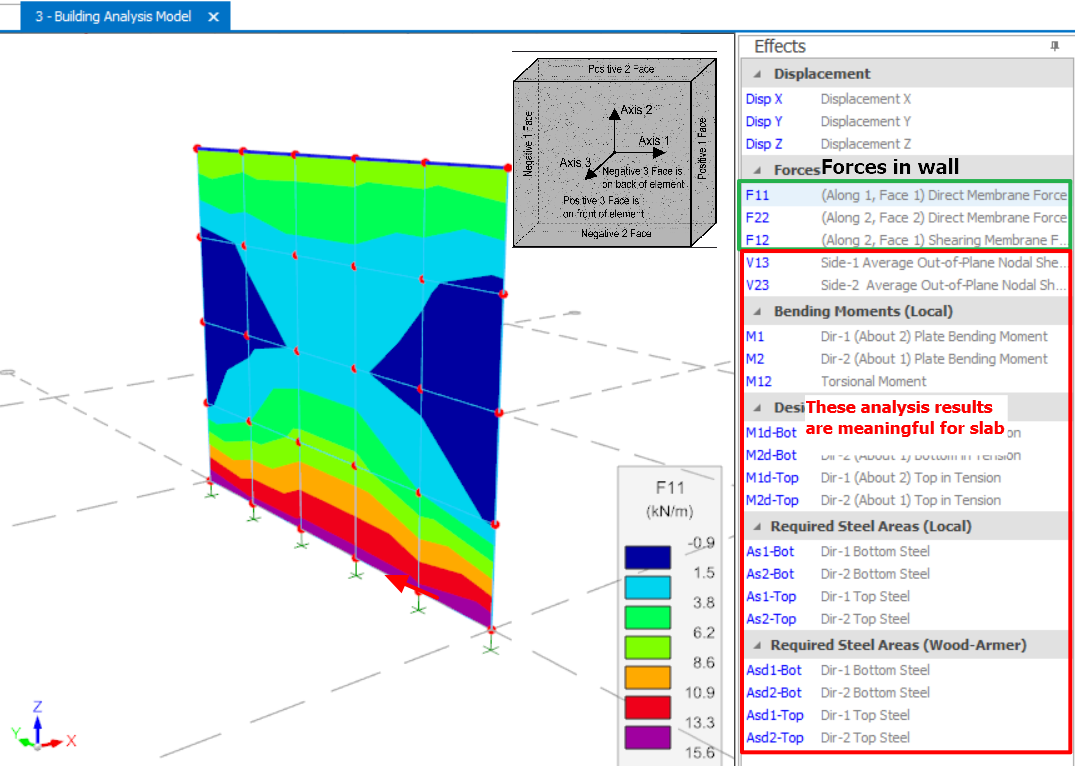
Snapshot below shows an example of FE shear wall contour. You can view the forces of F11, F22, F12, etc. of the shear wall.
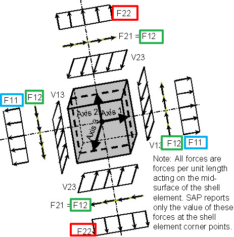
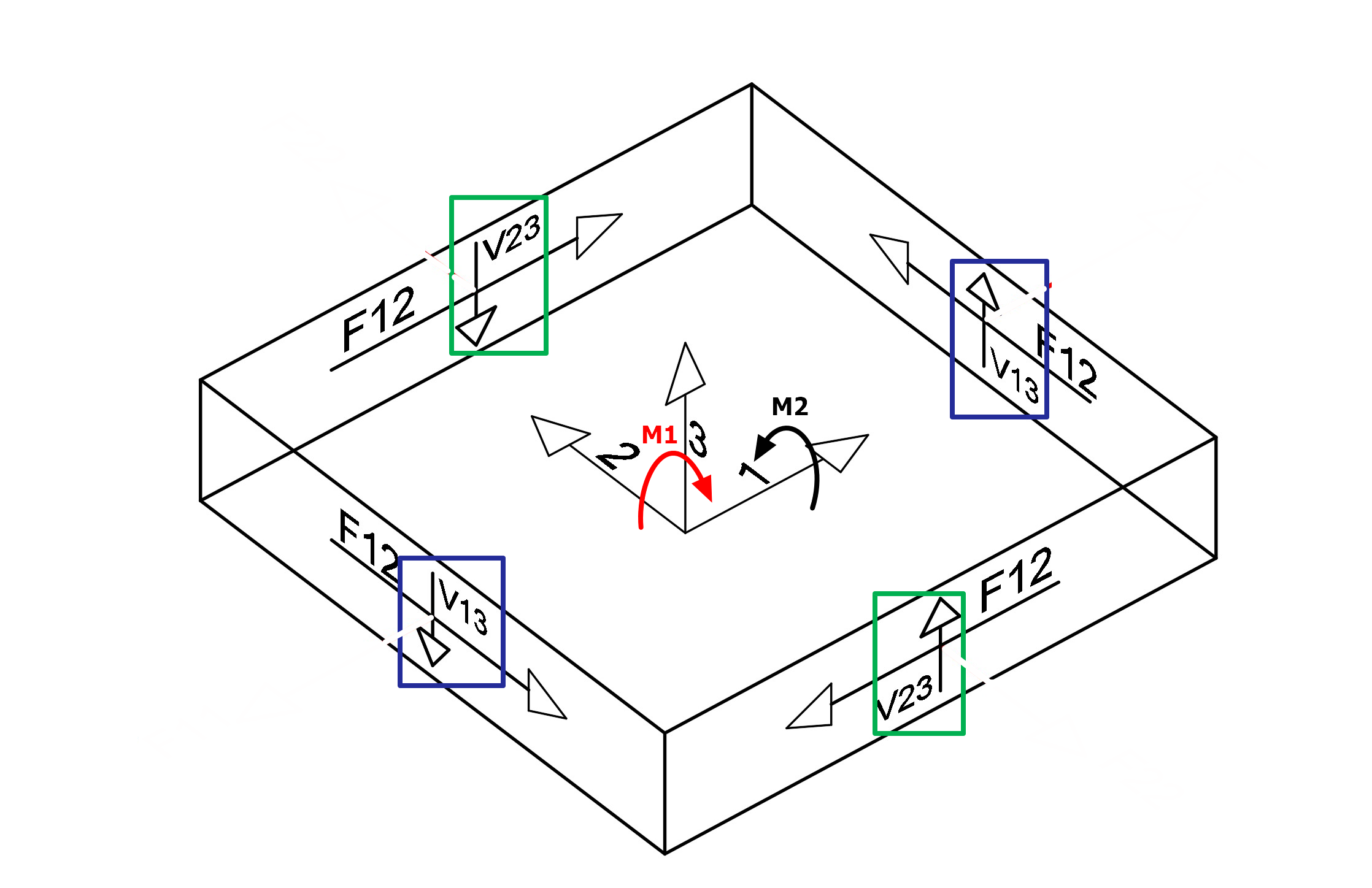
Image below is the sign convention of shell element to interpret the internal forces in the wall. Please note that the axes used for internal forces are local axes.
F11 – Direct Membrane Force at face 1 along direction 1.
F22 – Direct Membrane Force at at face 2 along direction 2.
F12 – Shearing Membrane Force at face 1 along direction 2.
V13 – Average Out-of-Plane Nodal Shear at Side 1
V23 – Average Out-of-Plane Nodal Shear at Side 2
M1 – Plate Bending Moment along local Direction-1 per unit length.
M2 – Plate Bending Moment along local Direction-2 per unit length.
M12 – Torsional / Twisting Moment per unit length.
ProtaStructure interpolates contour lines from the results on joints at each corner of the shells. Hence, the mesh sensitivity should be considered when interpreting and comparing the results. Mesh size can be controlled via the “Building Analysis > Model Options > "Shearwall Model".
Resultant forces derivation of Shearwall using FE Shells
Examining the individual shell forces is helpful if you want to visualize or compare forces of shearwalls of the model. However, the shell values cannot be directly used for wall design, as all the shell forces must be summed up correctly, to derive a total resultant value for axial, shear and moment force respectively.
To achieve this, ProtaStructure automatically utilizes the Group Sum methodology to calculate the total responses, i.e. total forces at the
top and bottom of the shearwalls modeled with FE shell elements :
This method calculates
the resultant of the joint forces at the shell elements and represents them on the geometrical center of
the shearwall or corewall.
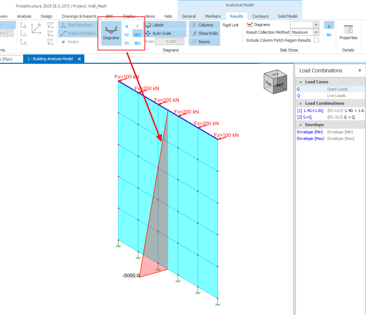
The resultant forces can be viewed in same manner as Mid-Pier Shearwall assumption, by going to Results tab > "Diagrams" > pick N, V2, V3, M22, M33 (example below)
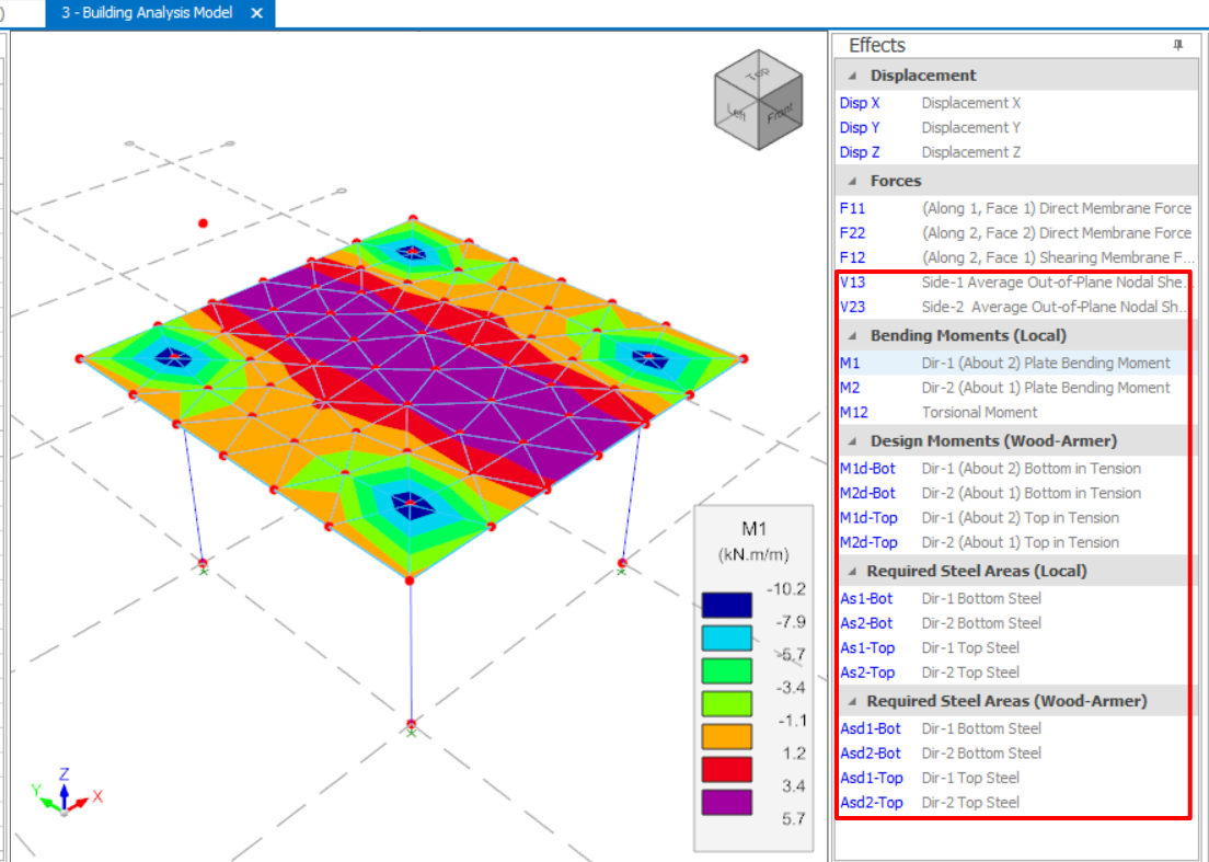
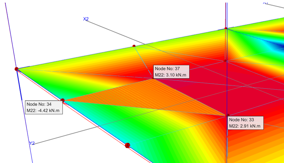
Snapshot below shows an example of FE slab contour. You can view the analysis results contour of shear forces, bending moments and area of steel required in the slab.
V13 is out of plane shear force at face 1 acting towards local axis 3.
V23 is out of plane shear force at face 2 acting towards local axis 3.
M1is Moment about Direction-1 per unit length.
M2is Moment about Direction-2 per unit length.
M12is Twisting Moment per unit length.
If you are running FE Floor Analysis instead of Building Analysis, you can refer to Finite Elements Floor Analysis article.
Additional User Interaction in Analytical Model
In the latest release ProtaStructure 2025, there are significant enhancements to user interactions in the Analytical Post Processor.
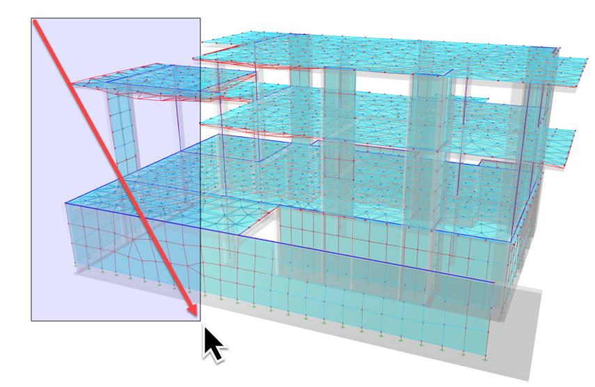
Window Selection
You can now select a part of the model by boxing around them.
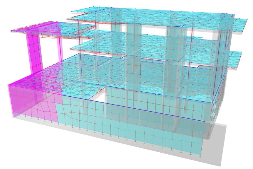
Isolating Selected Members
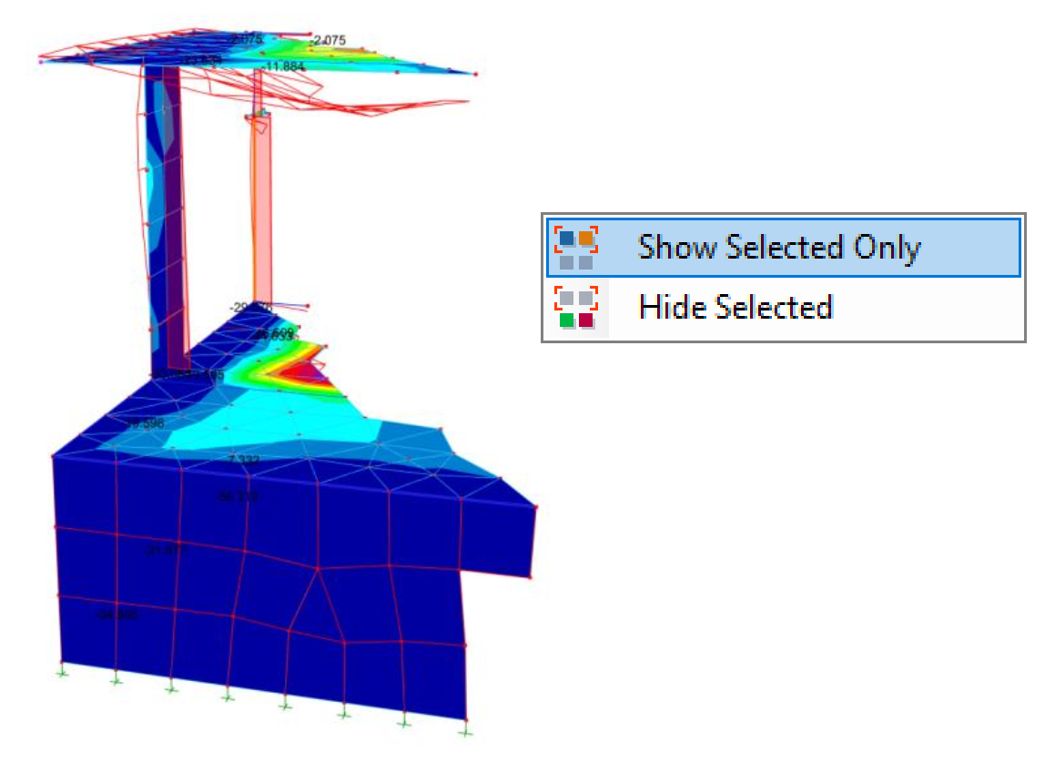
After selecting one or more members with window selection, right click and pick Show Selected Onlycommand. The results will be displayed only for selected part of the model.
To view the entire model again, right click and pick Show All command.
Hiding the Selected Members
Instead of showing only the selected members, you can choose to hide them. For that purpose, select one or more members, right click and pick Hide Selected command.
In the picture below, the moment diagram is displayed only for the selected frames.
In the example below, corner storey nodes are selected and only their displacement values are shown.
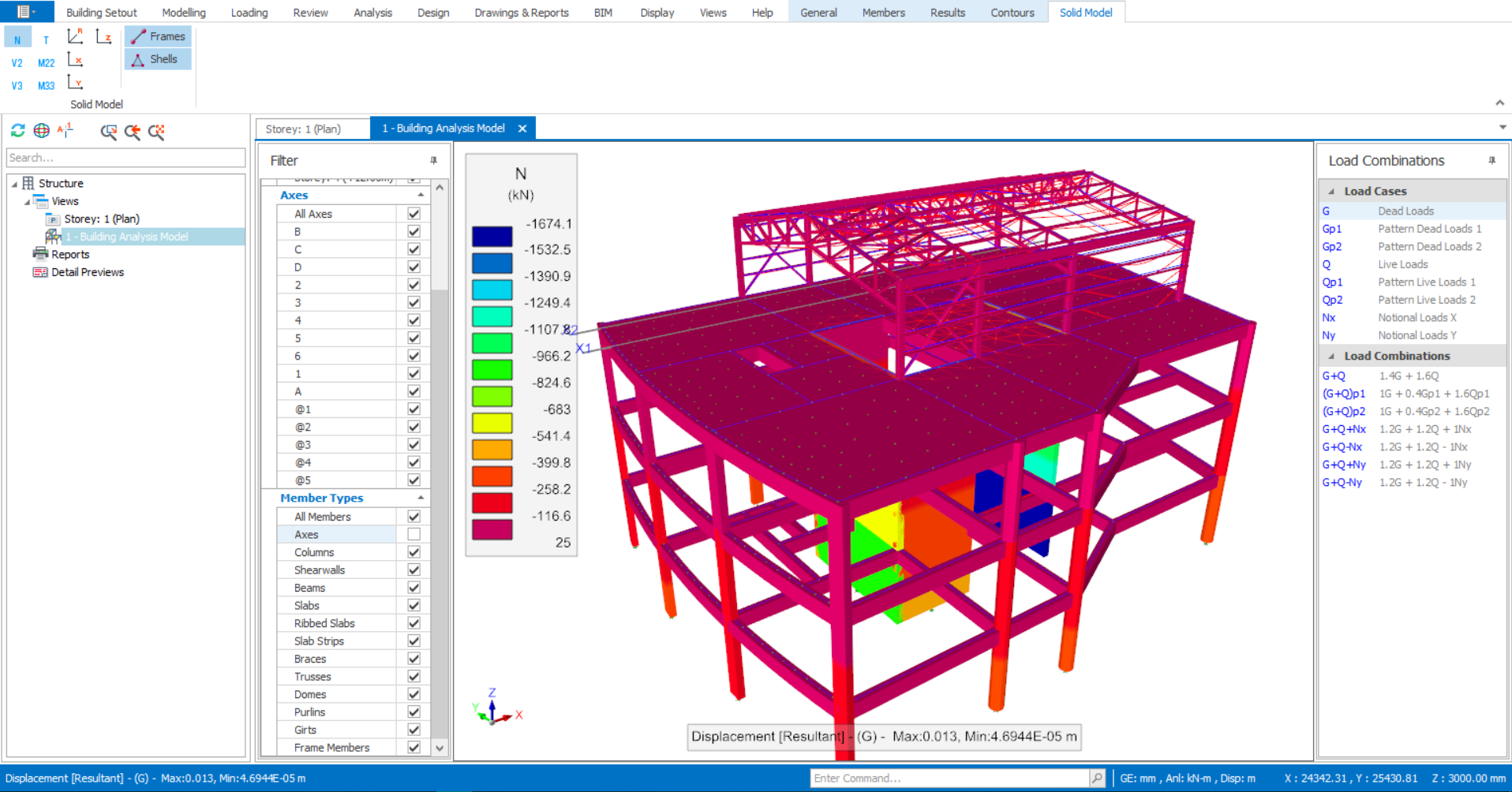
Solid Model
This allows various reactions such as axial load, shear force and bending moment are color coded shown on the physical model.
We use cookies to run the site, understand how it is used, and — with your permission — to measure our marketing. You decide which cookies to allow. Read our Privacy & Cookie Policy.
Manage cookie preferences
Strictly NecessaryAlways Active
Required for the website to work — navigation, security, and remembering your privacy choices. These cannot be switched off.
Analytics
Help us understand how visitors use the site so we can improve it. Data is aggregated.
Marketing
Used to measure our advertising and show you more relevant content across websites.



 Hence, when modelling, you need to ensure that members are using common axes or intersection of axes for members to be connected. Merely checking the 3D rendered view does not confirm whether members are connected analytically.
 –> Click to enlarge picture





 Press CTRL + F to call out this feature.

















 The Contours icons here is identical to the FE Floor Model (from FE Floor Analysis, kindly refer to this article : Finite Elements Floor Analysis